Quick start guide for new users
Step 1: Sign up an Amazon Web Service (AWS) account
Go to http://aws.amazon.com, click on “Create an AWS account” on the upper-right corner:

(the button will become “Sign In to the Console” for the next time)
After entering some basic information, you will be required to enter your credit card number. Don’t worry, this beginner tutorial will only cost you $0.1.
Note
If you are a student, check out the $100 educational credit (can be renewed every year!) at https://aws.amazon.com/education/awseducate/. I haven’t used up my credit for after playing with AWS for a whole year, so haven’t actually paid any money to them 😉
Now you should have an AWS account! It’s time to run the model in cloud. (You can skip Step 1 for the next time, of course)
Step 2: Launch a server with GEOS-Chem pre-installed
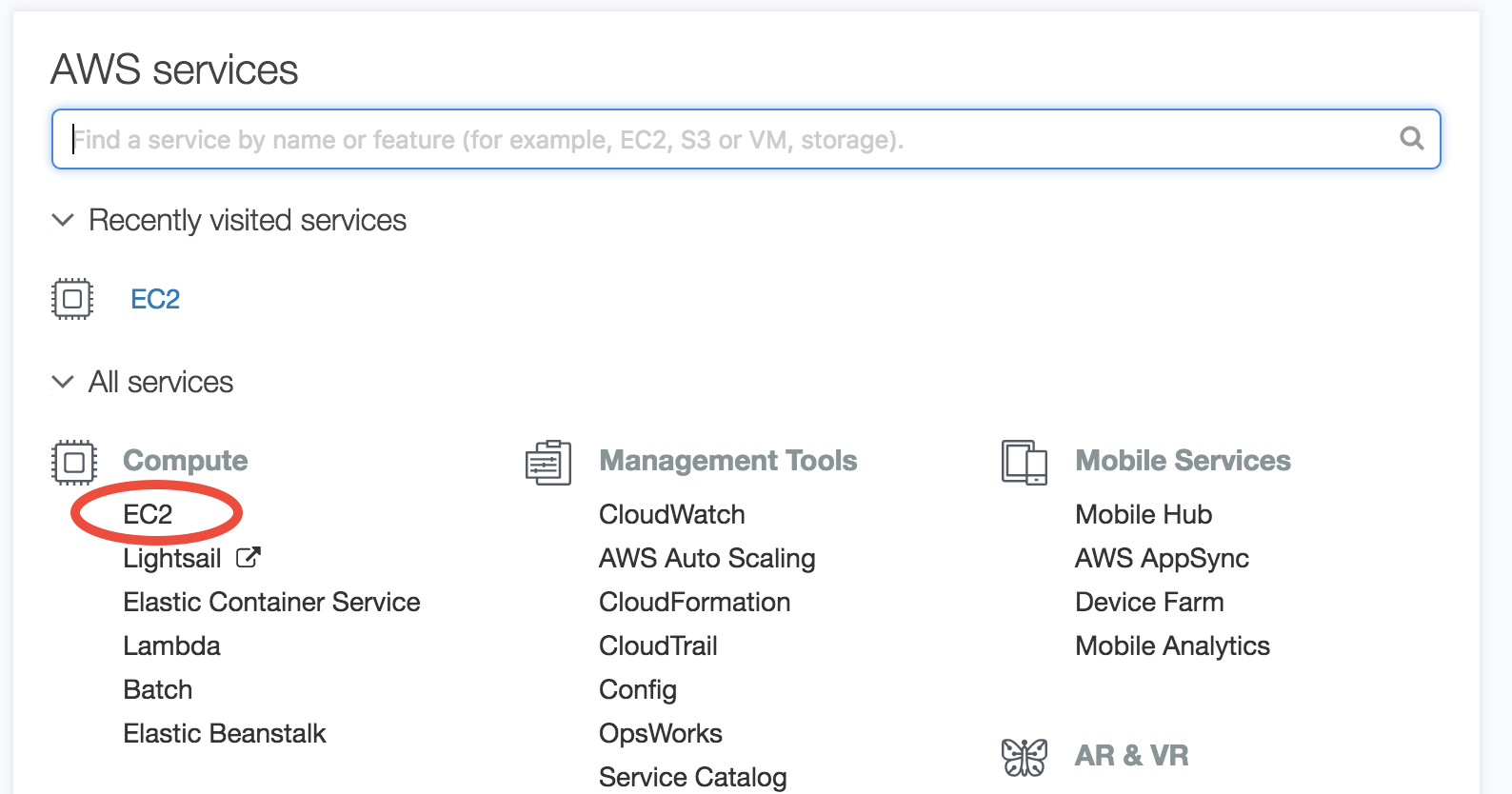
Log in to AWS console, and click on EC2 (Elastic Compute Cloud), which is the most basic cloud computing service.
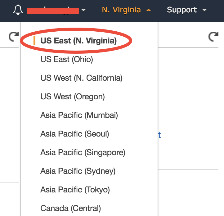
In the EC2 console, make sure you are in the US East (N. Virginia) region as shown in the upper-right corner of your console. Choosing a region closer to your physical location will give you better network. To keep this tutorial minimal, I built the system in only one region. But working across regions is not hard.
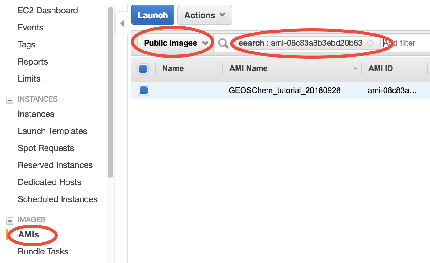
In the EC2 console, click on “AMI” (Amazon Machine Image) under “IMAGES” on the left navigation bar. Then select “Public images” and search for ami-08c83a8b3ebd20b63 or GEOSChem_tutorial_20180926 – that’s the system with GEOS-Chem installed. Select it and click on “Launch”.
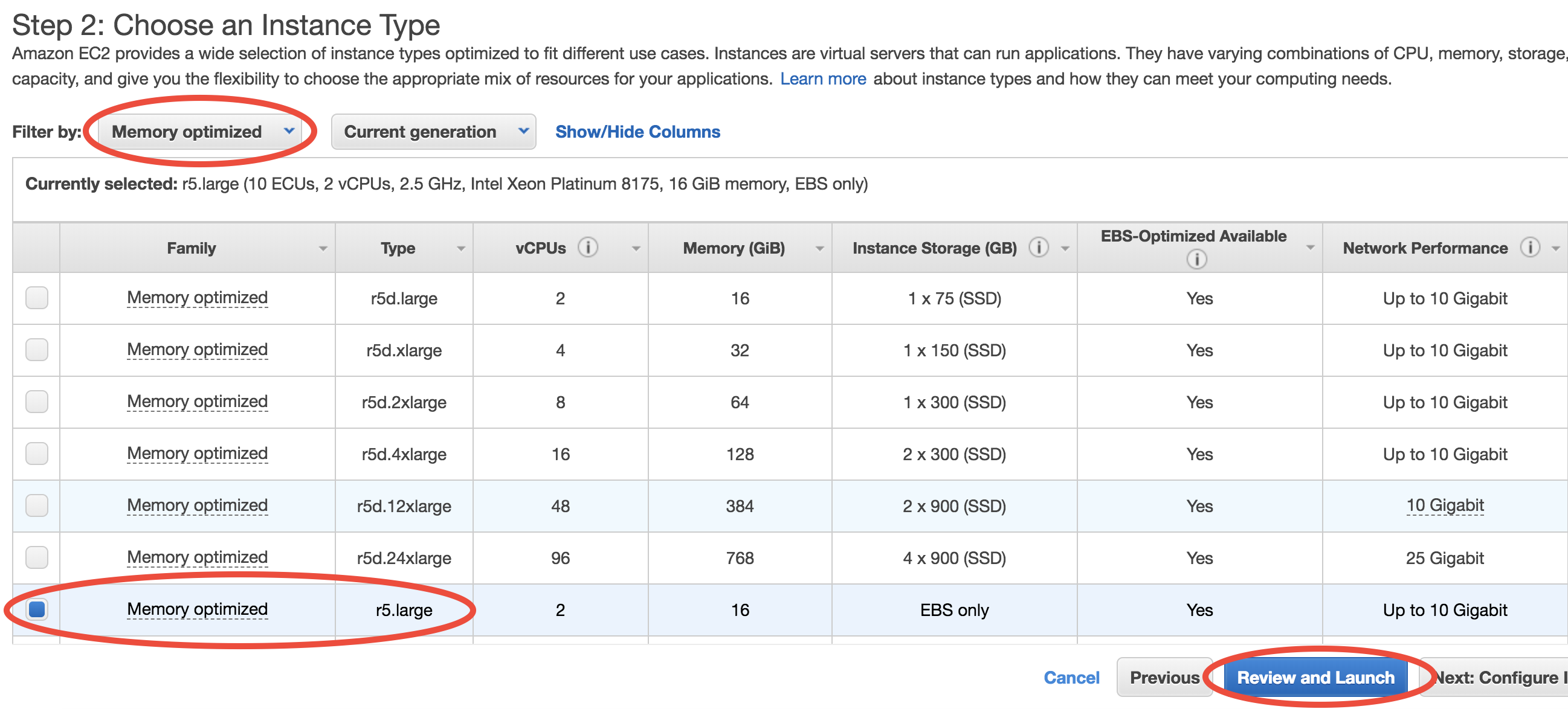
An AMI full specifies the “software” side of your virtual server, including the operating system, software libraries, and default data files. Then it’s time to specify the “hardware” side, mostly about CPUs.
You can select from a large number of CPU types at “Step 2: Choose an Instance Type”. In this toy example, choose “Memory optimized”-“r5.large” which meets the minimal hardware requirement for GEOS-Chem:
Then, just click on “Review and Launch”. You don’t need to touch other options this time. This brings you to “Step 7: Review Instance Launch”. Simply click on the Launch button again.
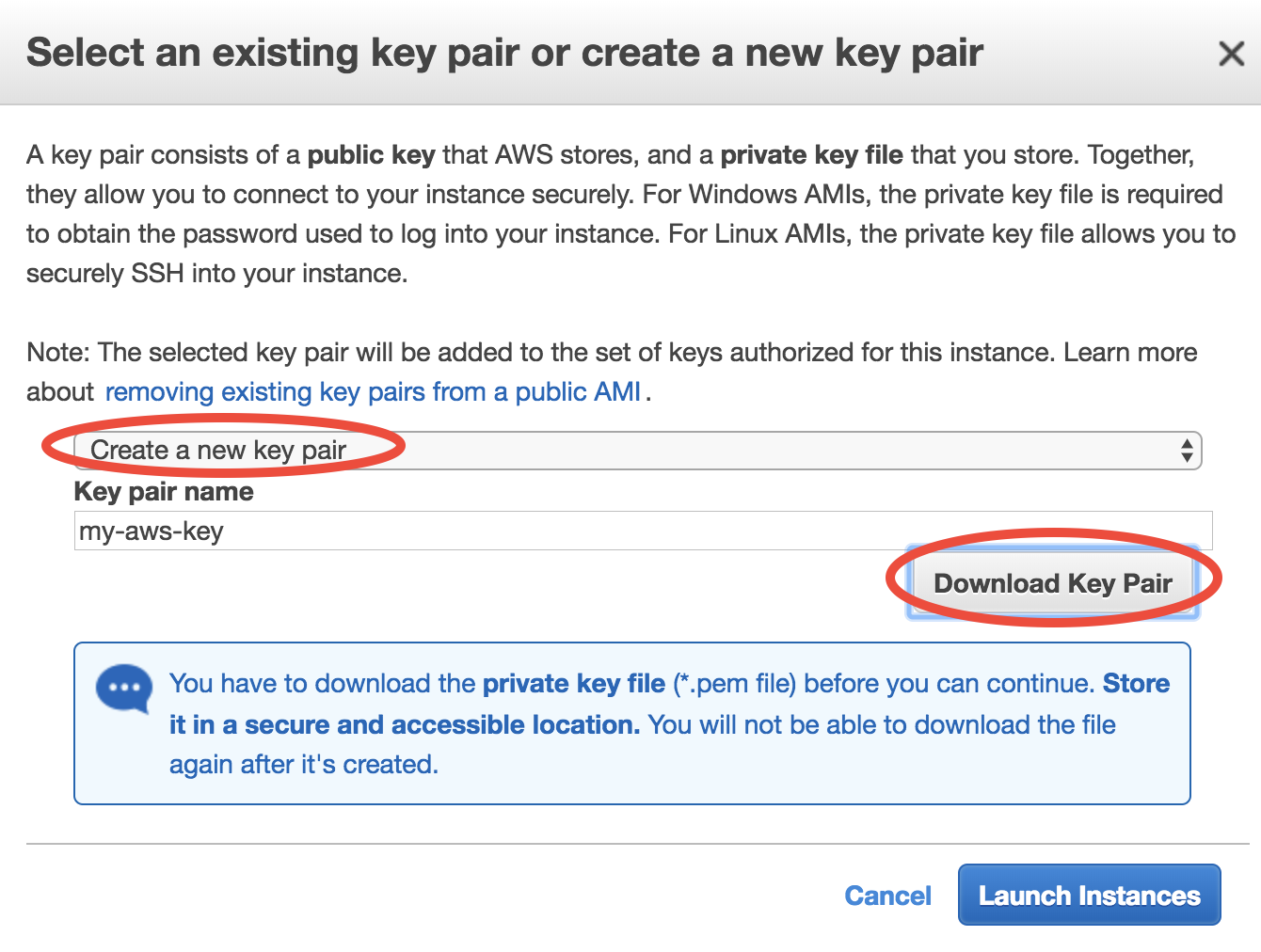
For the first time of using EC2, you will be asked to create and download a file called “Key Pair”. It is equivalent to the password you enter to ssh to your local server, but much more secure.
Give your “Key Pair” a name, click on “Download Key Pair”, and finally click on “Launch Instances”. (for the next time, you can simply select “Choose an existing Key Pair” and launch).
You can monitor your server in the EC2-Instance console. Within < 1min of initialization, “Instance State” should become “running”:
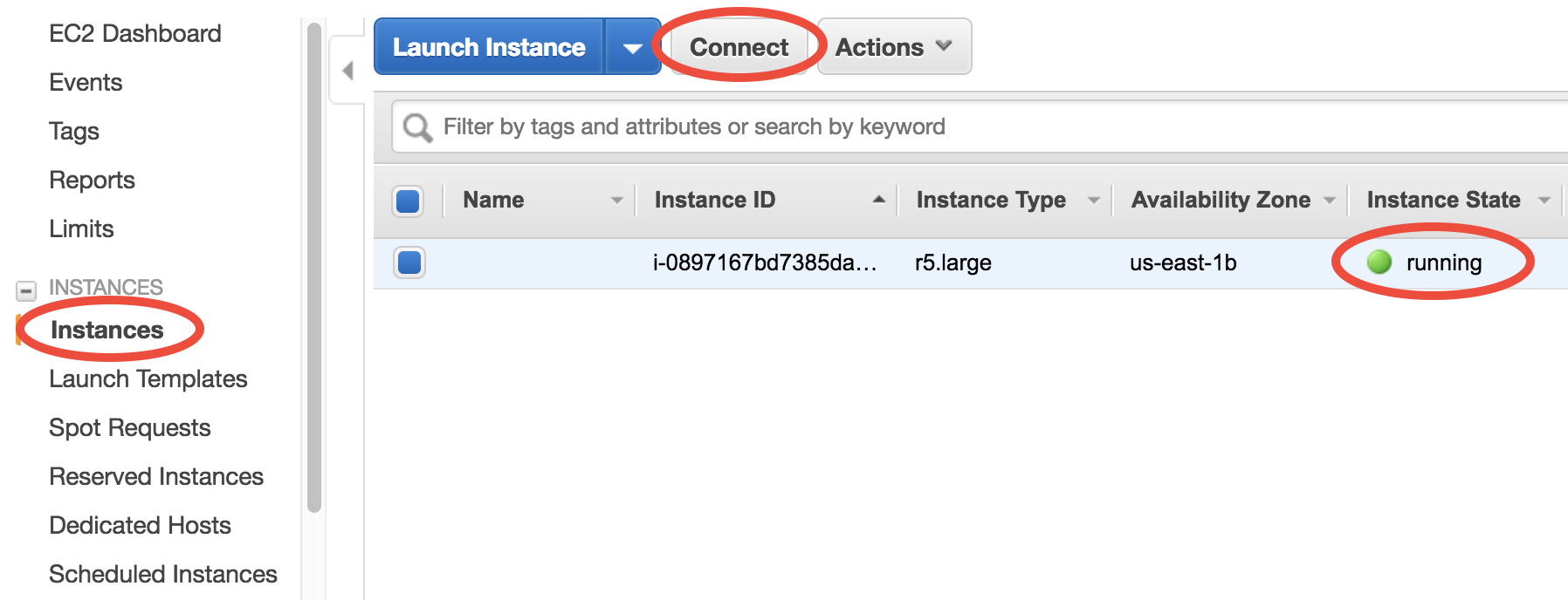
You now have your own server running on the cloud!
Step 3: Log into the server and run GEOS-Chem
Select your instance, click on the “Connect” button (shown in the above figure) near the blue “Launch Instance” button, then you should see this instruction page:
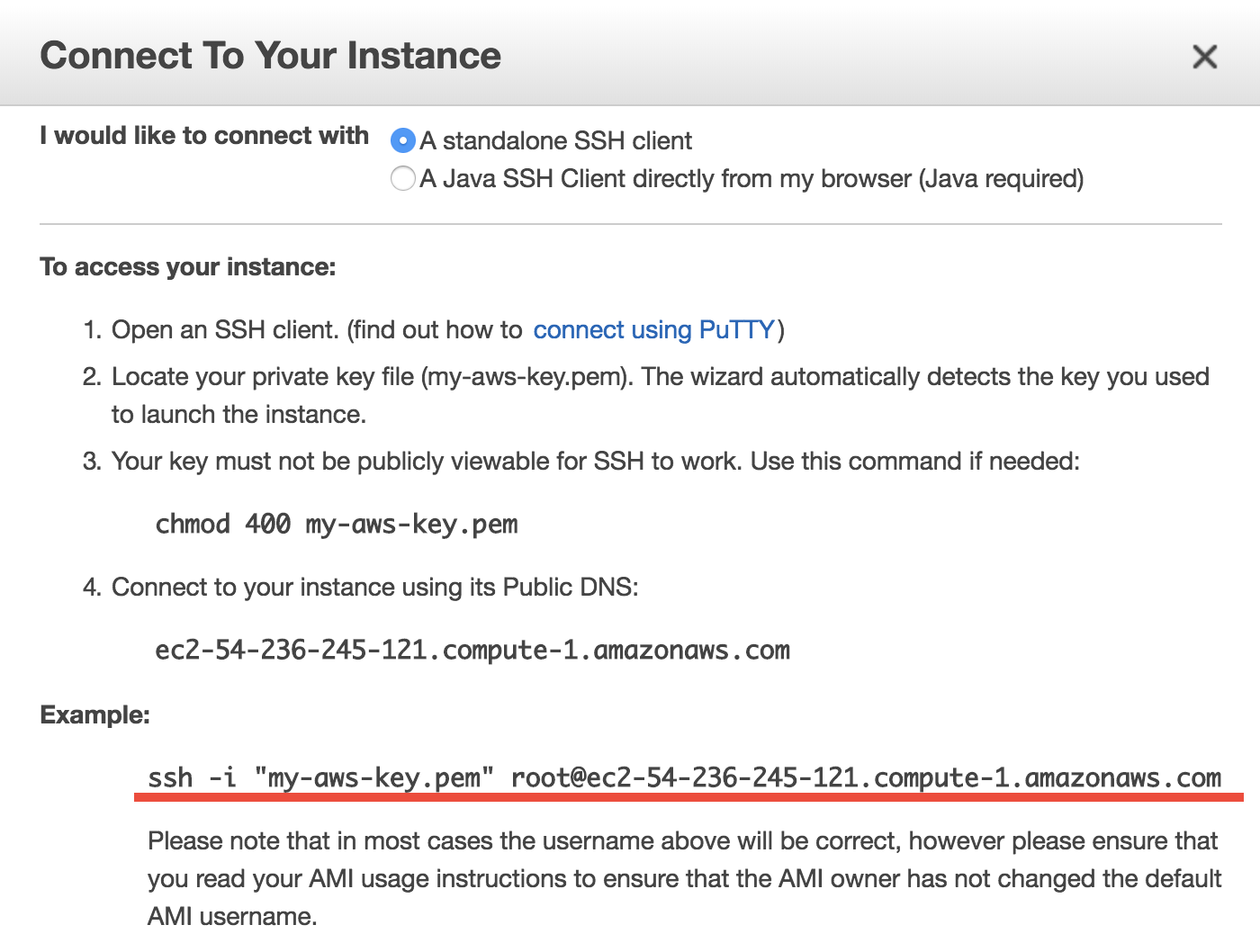
- On Mac or Linux, copy the
ssh -i "xx.pem" root@xxx.comcommand under “Example”. Before using that command to ssh to your server, do some minor stuff:cdto the directory where store your Key Pair (preferably$HOME/.ssh)- Use
chmod 400 xx.pemto change the key pair’s permission (also mentioned in the above figure; only need to do this at the first time). - Change the user name in that command from
roottoubuntu. (You’ll be asked to useubuntuif you keeproot).
- On Windows, please refer to the guide for MobaXterm and Putty (MobaXterm should be a lot easier). Alternatively, you can use the Windows Subsystem for Linux and then simply follow the above steps for Mac/Linux.
Your terminal should look like this:
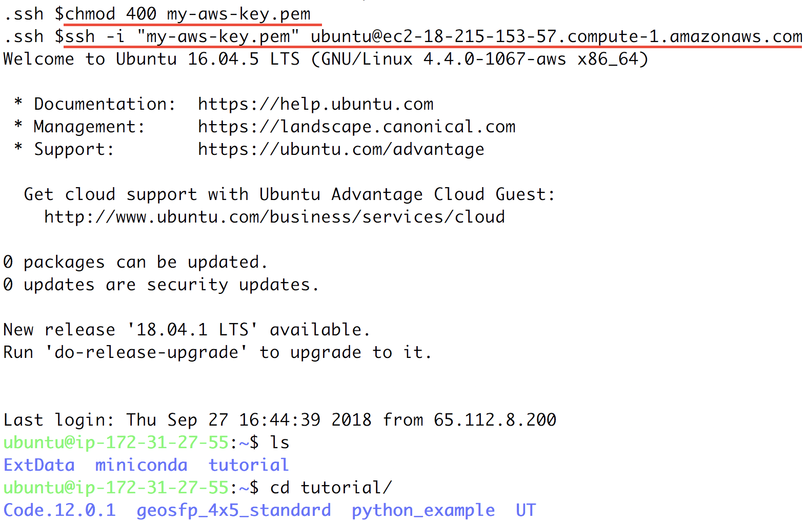
That’s a system with GEOS-Chem already built!
Note
Trouble shooting: if you have trouble ssh to the server, please make sure you don’t mess-up the “security group” configuration.
Go to the pre-generated run directory:
$ cd ~/tutorial/geosfp_4x5_standard
Just run the pre-compiled the model by:
$ ./geos.mp
Or you can re-compile the model on your own:
$ make realclean
$ make -j4 mpbuild NC_DIAG=y BPCH_DIAG=n TIMERS=1
Congratulations! You’ve just done a GEOS-Chem simulation on the cloud, without spending any time on setting up your own server, configuring software environment, and preparing model input data!
The default simulation length is only 20 minutes, for demonstration purpose. The “r5.large” instance type we chose has only a single, slow core (so it is cheap, just ~$0.1/hour), while its memory is large enough for GEOS-Chem to start. For serious simulations, it is recommended to use “Compute Optimized” instance types with multiple cores such as “c5.4xlarge”.
Note
The first simulation on a new server will have slow I/O and library loading because the disk needs “warm-up”. Subsequent simulations will be much faster.
Note
This system is a general environment for GEOS-Chem, not just a specific version of the model. This pre-configured run directory in the “tutorial” folder is only for demonstration purpose. Later tutorials will show you how to set up custom versions and configurations.
Step 4: Analyze output data with Python (Optional)
If you wait for the simulation to finish (takes 5~10 min), it will produce NetCDF diagnostics called GEOSChem.SpeciesConc.20160701.nc4 inside OutputDir/ of the run directory. To save time, you can also cancel the simulation and use the pre-generated file with the same name:
$ cd ~/tutorial/geosfp_4x5_standard/OutputDir/
$ ncdump -h GEOSChem.SpeciesConc.20160701_0000z.nc4
netcdf GEOSChem.SpeciesConc.20160701_0000z {
dimensions:
      time = UNLIMITED ; // (1 currently)
      lev = 72 ;
      ilev = 73 ;
      lat = 46 ;
      lon = 72 ;
variables:
      double time(time) ;
              time:long_name = "Time" ;
    time:units = "minutes since 2016-07-01 00:00:00 UTC" ;
              time:calendar = "gregorian" ;
              time:axis = "T" ;
...
Anaconda Python and xarray are already installed on the server for analyzing all kinds of NetCDF files. If you are not familiar with Python and xarray, checkout my Python/xarray tutorial for GEOS-Chem users.
Activate the pre-installed geoscientific Python environment by source activate geo (it is generally a bad idea to directly install things into the root Python environment), and then start ipython from the command line:
$ source activate geo  # I also set a `act geo` alias
$ ipython
Python 3.6.6 |Anaconda, Inc.| (default, Jun 28 2018, 17:14:51)
Type 'copyright', 'credits' or 'license' for more information
IPython 6.5.0 -- An enhanced Interactive Python. Type '?' for help.

In [1]: import xarray as xr

In [2]: ds = xr.open_dataset('GEOSChem.SpeciesConc.20160701_0000z.nc4')

In [3]: ds
Out[3]:
<xarray.Dataset>
Dimensions:         (ilev: 73, lat: 46, lev: 72, lon: 72, time: 1)
...
    SpeciesConc_CO  (time, lev, lat, lon) float32 ...
    SpeciesConc_O3  (time, lev, lat, lon) float32 ...
    SpeciesConc_NO  (time, lev, lat, lon) float32 ...
A much better data-analysis environment is Jupyter notebooks. If you have been using Jupyter on your local machine, the user experience on the cloud would be exactly the same.
To use Jupyter on remote servers, re-login to the server with port-forwarding option -L 8999:localhost:8999:
$ ssh -i "xx.pem" ubuntu@xxx.com -L 8999:localhost:8999
Then simply run jupyter notebook --NotebookApp.token='' --no-browser --port=8999:
$ source activate geo
$ jupyter notebook --NotebookApp.token='' --no-browser --port=8999
[I 21:11:41.503 NotebookApp] Writing notebook server cookie secret to /run/user/1000/jupyter/notebook_cookie_secret
[W 21:11:41.986 NotebookApp] All authentication is disabled.  Anyone who can connect to this server will be able to run code.
[I 21:11:42.046 NotebookApp] Serving notebooks from local directory: /home/ubuntu
[I 21:11:42.046 NotebookApp] 0 active kernels
[I 21:11:42.046 NotebookApp] The Jupyter Notebook is running at:
[I 21:11:42.046 NotebookApp] http://localhost:8999/
[I 21:11:42.046 NotebookApp] Use Control-C to stop this server and shut down all kernels (twice to skip confirmation).
Visit http://localhost:8999/ in your browser, you should see a Jupyter environment just like on local machines. The server contains an example notebook that you can just execute. It is located at:
~/tutorial/python_example/sample-python-code.ipynb
Besides being a data analysis environment, Jupyter can also be used as a graphical text editor on remote servers so you don’t have to use vim/emacs/nano. The Jupyter console also allows you to download/upload data without using scp. The next generation of notebooks, namely Jupyter Lab, is also installed. Just change the launching command from jupyter notebook ... to jupyter lab ... if you want to have a try.
Note
There are many ways to connect to Jupyter on remote servers. Port-forwarding is the easiest way, and is the only way that also works on local HPC clusters (which has much stricter firewalls than cloud platforms). The port number 8999 is just my random choice, to distinguish from the default port number 8888 for local Jupyter. You can use whatever number you like as long as it doesn’t conflict with existing port numbers.
We encourage users to try the new NetCDF diagnostics, but you can still use the old BPCH diagnostics if you want to. Just compile with NC_DIAG=n BPCH_DIAG=y instead. The Python package xbpch can read BPCH data into xarray format, so you can use very similar code for NetCDF and BPCH output. xbpch is pre-installed in the geo environment. My xESMF package is also pre-installed, which can fulfill almost all horizontal regridding needs for GEOS-Chem data (and most of Earth science data).
Also, you could indeed download the output data and use old tools like IDL & MATLAB to analyze them, but we highly recommend the open-source Python/Jupyter/xarray ecosystem. It will vastly improve user experience and working efficiency, and also help open science and reproducible research.
Step 5: Shut down the server (Very important!!)
Right-click on the instance in your console to get this menu:
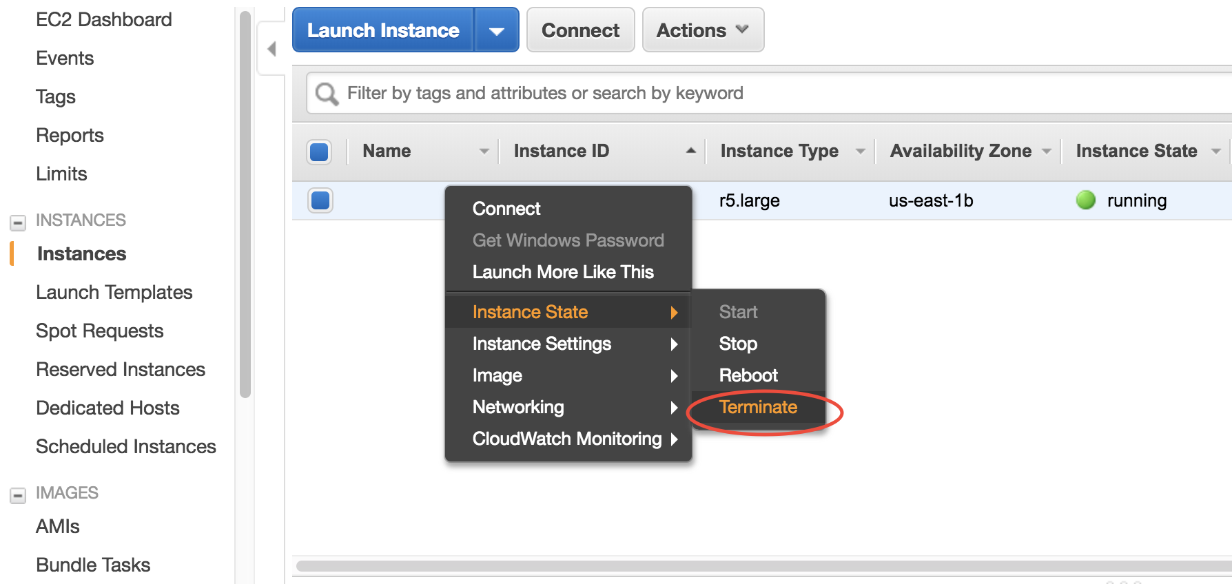
There are two different ways to stop being charged:
- “Stop” will make the system inactive, so that you’ll not be charged by the CPU time, but only be charged by the negligible disk storage fee. You can re-start the server at any time and all files will be preserved.
- “Terminate” will completely remove that virtual server so you won’t be charged at all after that. Unless you save your system as an AMI or transfer the data to other storage services, you will lose all your data and software.
You will learn how to save your data and configurations persistently in the next tutorials. You might also want to simplify your ssh login command.